There are two kinds of Excel users: people who have used VLOOKUP, and people who have stared at a sprea classic Excel function that connects related data, saving you from manually copying values row by row like it is 1997 and your mouse has a roller ball.
Whether you are matching employee IDs to departments, product codes to prices, customer names to email addresses, or test scores to letter grades, VLOOKUP can pull the right information from a reference table in seconds. It is not perfect, and newer functions such as XLOOKUP have improved on some of its limitations. Still, VLOOKUP remains one of the most useful Excel formulas to understand, especially when you work with older spreadsheets, shared templates, or reports built by someone who considers “Final_Final_UseThisOne.xlsx” a reasonable filename.
This guide explains how to use VLOOKUP in Excel step by step, including exact matches, approximate matches, common errors, practical examples, and a few hard-earned lessons that can keep your spreadsheet from becoming an accidental work of fiction.
What Is VLOOKUP in Excel?
VLOOKUP stands for Vertical Lookup. It searches for a value in the first column of a selected table and returns related information from another column in the same row.
For example, imagine you have a product ID in one worksheet and a product catalog in another. Instead of manually typing each product price, you can use VLOOKUP to search for the product ID and return the corresponding price automatically.
In simple terms, VLOOKUP tells Excel:
“Find this value in the first column of my table, then bring back something from the same row.”
That is the heart of the function. The rest is just teaching Excel where to look and what to bring home.
The VLOOKUP Formula Syntax
The standard VLOOKUP formula looks like this:
It looks intimidating at first, but each argument has a very specific job.
1. lookup_value
This is the value you want Excel to find. It might be a customer ID, employee number, SKU, email address, state abbreviation, or any other unique identifier.
For example, if cell A2 contains a product code, your lookup value might be:
2. table_array
This is the table or cell range where Excel will search. The lookup value must be located in the first column of this selected range.
For example:
The dollar signs lock the table range so it does not move when you copy the formula down. Without them, Excel may wander off into the spreadsheet wilderness and return results from the wrong place.
3. col_index_num
This number tells Excel which column to return from within the selected table range.
Suppose your table range is F2:H20:
| Column in Range | Spreadsheet Column | Example Data |
|---|---|---|
| 1 | F | Product ID |
| 2 | G | Product Name |
| 3 | H | Price |
If you want the product name, use 2. If you want the price, use 3.
Excel counts columns inside the selected table range, not columns across the entire worksheet. That small detail has launched approximately one million confused stares at column letters.
4. range_lookup
This final argument determines whether Excel should find an exact match or an approximate match.
FALSEmeans find an exact match.TRUEmeans find an approximate match.
For most everyday uses of VLOOKUP, choose FALSE. Exact matching is ideal for employee IDs, invoice numbers, product codes, usernames, customer accounts, and other data that should match precisely.
Use TRUE only when you are working with sorted threshold values, such as tax brackets, commission ranges, shipping tiers, or grading scales.
How to Use VLOOKUP: A Simple Step-by-Step Example
Let’s say you have an order sheet with product IDs but no product names or prices. On another worksheet, called Product List, you have a reference table with product IDs, names, and prices.
Example Data
Your order worksheet might look like this:
| Product ID | Product Name | Price |
|---|---|---|
| P1001 | ||
| P1002 | ||
| P1003 |
Your Product List worksheet contains:
| Product ID | Product Name | Price |
|---|---|---|
| P1001 | Wireless Mouse | $24.99 |
| P1002 | USB Keyboard | $39.99 |
| P1003 | Webcam | $59.99 |
Step 1: Click the First Result Cell
Click the first blank cell where you want the product name to appear. In this example, that would be cell B2 on the order worksheet.
Step 2: Enter the VLOOKUP Formula
Type the following formula:
Here is what it means:
A2is the product ID you want to find.'Product List'!$A$2:$C$100is the reference table on another worksheet.2tells Excel to return the value from the second column of that table.FALSEtells Excel to find an exact product ID match.
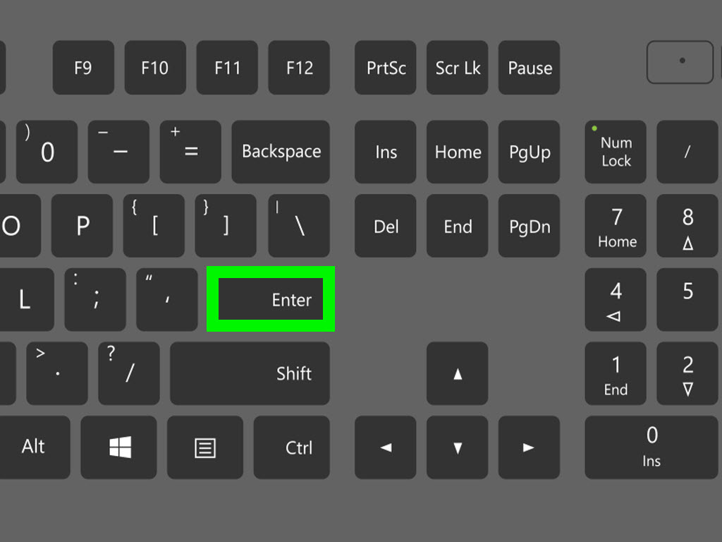
Press Enter. Excel should return Wireless Mouse.
Step 3: Pull the Formula Down
Click the cell containing the formula. Then drag the small square in the bottom-right corner down through the rest of the rows. Excel will update the lookup value automatically for each row.
To return the product price in column C, use:
That single formula can fill hundreds or thousands of rows. It is one of those Excel moments that makes you feel like a wizard, even though you mostly just used commas correctly.
Using VLOOKUP for an Exact Match
An exact-match VLOOKUP is the version most people use. It looks for one specific value and returns the associated data only when it finds a perfect match.
Use exact match VLOOKUP for:
- Employee IDs
- Customer account numbers
- Product SKUs
- Invoice numbers
- Student IDs
- Membership numbers
- Email addresses
Here is a common employee lookup example:
Suppose column A contains employee IDs, and columns F through H contain employee ID, department, and manager. This formula finds the ID in A2 and returns the manager from the third column of the selected table.
Always include FALSE when you need an exact match. Leaving out the final argument can cause Excel to use approximate matching, which is not the kind of surprise anyone wants in a payroll report.
Using VLOOKUP for an Approximate Match
Approximate match VLOOKUP is useful when the exact number does not appear in your table, but you want Excel to return the closest value without going over.
A grading scale is a classic example.
| Minimum Score | Letter Grade |
|---|---|
| 0 | F |
| 60 | D |
| 70 | C |
| 80 | B |
| 90 | A |
If a student’s score is in cell B2, you could use:
If B2 contains 87, Excel finds the closest lower threshold, which is 80, and returns B.
There is one major rule: the first column of an approximate-match table must be sorted in ascending order. If it is not sorted correctly, Excel can return an incorrect result with the confidence of a toddler wearing sunglasses indoors.
Common VLOOKUP Errors and How to Fix Them
#N/A Error
The #N/A error means Excel could not find the lookup value. This is the most common VLOOKUP issue.
Possible causes include:
- The lookup value does not exist in the reference table.
- There is an extra space before or after a value.
- One list stores values as text, while the other stores them as numbers.
- The selected table range does not include the needed record.
- You used
FALSEbut the values are not identical.
To display a friendlier message instead of #N/A, wrap your formula in IFERROR:
This is useful for reports shared with coworkers who may not appreciate a spreadsheet that appears to be yelling in code.
#REF! Error
A #REF! error usually means the column index number is too large for the selected table range.
For example, this formula will fail:
The selected range contains only three columns: F, G, and H. Asking for column 4 is like asking a three-story building where the fourth floor is. Excel has no answer, and frankly, neither do architects.
Wrong Results
If VLOOKUP returns a value but it is not the right one, check whether you accidentally used TRUE instead of FALSE. Approximate match can return nearby values, which is helpful for grading scales but dangerous for customer records.
Numbers Stored as Text
Excel may treat something that looks like a number as text. This often happens when data is imported from a website, accounting platform, CSV file, or another person’s spreadsheet that has seen too many revisions.
Try converting both lookup columns to the same format. You can use Excel’s warning icon, Text to Columns, VALUE, or paste special options to clean the data.
Best Practices for Using VLOOKUP in Excel
Use Unique Lookup Values
VLOOKUP returns the first matching value it finds. If your reference table contains duplicate product IDs or employee numbers, Excel will not ask which one you meant. It will simply choose the first match and move on with its day.
Whenever possible, use unique IDs as your lookup values.
Lock Your Table Range
Use absolute cell references with dollar signs when copying formulas down:
This keeps the reference table fixed while the lookup value changes from row to row.
Convert Your Reference List into an Excel Table
Excel Tables are useful because they expand automatically when you add new records. Select your data, press Ctrl + T, and assign a descriptive name such as ProductCatalog.
Your formula can then become:
This is easier to read and less likely to break when new products, employees, or customers are added.
Keep the Lookup Column on the Left
VLOOKUP can only search the first column of the selected range and return information to the right. It cannot look left.
For example, if your product ID is in column D but your price is in column B, VLOOKUP cannot retrieve the price unless you rearrange the table or use another function.
Use Clear Sheet Names
Names such as Data, Sheet2, and New Data Final make formulas harder to understand six months later. Use names like EmployeeDirectory, PricingTable, or CustomerMaster.
Your future self will be grateful. Your future coworker may even buy you coffee.
VLOOKUP Across Different Worksheets
VLOOKUP is especially helpful when information is stored on separate worksheets in the same workbook.
For instance, imagine:
- Your Sales Report sheet contains order numbers and customer IDs.
- Your Customer Database sheet contains customer IDs, names, email addresses, and regions.
To return the customer name from another worksheet, use a formula like this:
Excel looks for the customer ID in B2, searches column A of the Customer Database sheet, and returns the value from the second column of that range.
If the worksheet name contains spaces, place it inside single quotation marks. Excel is polite about spaces, but only when you remember the quotation marks.
Can You Use VLOOKUP Between Different Excel Workbooks?
Yes. VLOOKUP can retrieve information from another Excel workbook, although the formula becomes longer.
A basic cross-workbook formula may look like this:
This can be useful when one workbook contains master data, such as inventory details, vendor records, or approved pricing, while another workbook contains day-to-day transactions.
Keep in mind that external workbook links can become fragile if files are renamed, moved, or sent to someone else without the supporting workbook. When possible, keep linked files in a stable shared location and use clear file names.
VLOOKUP vs. XLOOKUP: Which Should You Use?
VLOOKUP is still widely used, but XLOOKUP is often more flexible in newer versions of Excel.
XLOOKUP can search in either direction, which means it can return values from columns to the left or right of the lookup column. It also uses exact match by default and allows you to specify what should happen when no result is found.
For example, an XLOOKUP formula might look like this:
That formula searches for the value in A2 within F2:F500 and returns the matching value from H2:H500. If there is no match, it displays “Not Found.”
Still, VLOOKUP remains valuable because many workplaces use older Excel versions, inherited reports, and templates built around it. Knowing VLOOKUP is a little like knowing how to use a can opener: newer gadgets exist, but this one still gets the job done.
Practical VLOOKUP Use Cases
VLOOKUP is useful in nearly every type of spreadsheet-driven work. Here are a few practical examples:
Inventory Management
Match product codes to names, prices, supplier details, stock levels, reorder points, or warehouse locations.
Sales Reporting
Pull customer names, sales territories, account managers, commission rates, or product categories into order reports.
Human Resources
Match employee IDs to departments, job titles, managers, office locations, benefit categories, or training records.
Finance and Accounting
Retrieve tax rates, account descriptions, vendor details, expense categories, payment terms, or approved budget amounts.
Education
Match student IDs to names, class schedules, attendance records, scholarship information, or grade bands.
Experience-Based Tips for Working with VLOOKUP
VLOOKUP is one of those Excel functions that seems almost too simple once you understand it. The formula has only four arguments, and the basic version can be learned in a few minutes. The real experience comes later, when you are handed a workbook with 14 tabs, five hidden columns, three versions of the same customer list, and someone has formatted half the account numbers as text for reasons known only to the spreadsheet gods.
The first lesson is that VLOOKUP is often not the problem. The data is. When a formula returns #N/A, the instinct is to rewrite the formula repeatedly. In many cases, the formula is fine, but the data contains invisible spaces, mismatched formats, duplicate values, or a slightly different version of the lookup key. A product code that looks like AB-100 may actually be AB-100 with a trailing space. To the human eye, they are twins. To Excel, they are distant cousins who do not speak.
Before blaming the formula, compare the lookup value and the corresponding value in the reference table. Click into each cell and inspect the formula bar. Use TRIM() to remove extra spaces when needed. Check whether numeric values are stored as numbers in one list and text in another. Sometimes adding a leading apostrophe, importing from a CSV file, or copying from a website quietly changes the data type.
A second lesson is to avoid building formulas around names when a stable ID exists. People have duplicate names. Businesses have similar names. Products sometimes have names that change because marketing had a meeting. Unique IDs are much safer. A customer number, order ID, SKU, employee ID, or internal account code usually makes a better VLOOKUP key than a name.
Another practical habit is to test VLOOKUP with a few known records before filling the formula down thousands of rows. Pick one value you know should match, one value that should not match, and one value near the edge of the table. This small test can reveal whether your reference range is incomplete, your column index is wrong, or your match setting needs attention.
It is also worth treating the fourth VLOOKUP argument with respect. Many spreadsheet errors happen because the formula omits FALSE. Excel then assumes approximate matching, which can create incorrect results without obvious warning. That is especially risky in sales reports, payroll sheets, inventory files, and financial workbooks where “close enough” is not a valid accounting principle.
For approximate matches, use a clearly labeled threshold table and make sorting part of the workflow. A commission table, grade scale, or shipping rate schedule should be sorted from lowest threshold to highest threshold before you use TRUE. It helps to add a note near the table so the next person understands that rearranging rows can change the result.
When formulas start becoming difficult to read, named ranges and Excel Tables can make a major difference. Instead of pointing VLOOKUP at a mysterious range like $G$4:$J$1527, give the data a meaningful table name such as VendorRates or EmployeeRoster. The formula becomes easier to audit, easier to explain, and less likely to trigger a minor panic attack during a Monday morning report review.
Finally, remember that VLOOKUP is a tool, not a personality test. You do not need to memorize every Excel function before you use it. Start with a small lookup table, build one exact-match formula, verify the result, and copy it down. Once that feels comfortable, move on to error handling, approximate matches, other worksheets, and eventually XLOOKUP. Spreadsheet confidence grows one successful formula at a time.
Final Thoughts
Learning how to use VLOOKUP with an Excel spreadsheet can turn a messy collection of lists into a connected, useful dataset. Instead of manually searching for names, prices, departments, records, or categories, you can let Excel do the matching work for you.
Start with exact matches, use FALSE for most business data, lock your table range with dollar signs, and keep your lookup column on the left side of the selected table. Once you have those basics down, VLOOKUP becomes less of a mysterious formula and more of a reliable spreadsheet sidekick.
Note: Formula separators can vary by regional Excel settings. Some versions of Excel use semicolons instead of commas, so replace commas with semicolons if your formula is rejected even though the logic is correct.