Eigenvalues and eigenvectors sound like something a math professor whispers dramatically before lightning strikes the chalkboard. In reality, they are one of the most useful ideas in linear algebra. They help explain how a matrix transforms space, which directions stay steady, and how much those directions stretch, shrink, flip, or stay exactly the same.
Whether you are studying linear algebra, machine learning, engineering, physics, economics, computer graphics, or data science, learning how to calculate eigenvalues and eigenvectors in a matrix is a big step forward. The good news? The core process is surprisingly organized. Once you understand the recipe, the mystery fades faster than your calculator battery during finals week.
This guide explains eigenvalues and eigenvectors in plain American English, walks through the calculation steps, gives a complete matrix example, and shares practical tips from real problem-solving experience.
What Are Eigenvalues and Eigenvectors?
An eigenvector is a nonzero vector that keeps its direction when a matrix transformation is applied to it. It may get longer, shorter, reversed, or unchanged, but it remains on the same line. The eigenvalue is the number that tells you how the eigenvector is scaled.
The defining equation is:
Av = λv
Here, A is a square matrix, v is the eigenvector, and λ is the eigenvalue. In plain language, multiplying the matrix by the vector gives the same result as multiplying the vector by a scalar. That scalar is the eigenvalue.
A Simple Way to Think About It
Imagine a matrix as a machine that moves arrows around. Most arrows get rotated, stretched, or pushed into new directions. But a few special arrows do not change direction. Those are eigenvectors. The amount each special arrow is stretched or compressed is its eigenvalue.
If λ = 3, the eigenvector becomes three times as long. If λ = 1, it stays the same length. If λ = -1, it flips direction. If λ = 0, it collapses into the zero vector. In other words, eigenvalues are like the matrix’s personality test results.
Why Eigenvalues and Eigenvectors Matter
Eigenvalues and eigenvectors are not just classroom decorations. They show up in many real-world applications because they reveal the hidden structure of a matrix.
- Data science: Principal component analysis, or PCA, uses eigenvectors to find important directions in data.
- Engineering: Vibration analysis uses eigenvalues to study natural frequencies.
- Physics: Quantum mechanics uses eigenvalues to represent measurable quantities.
- Differential equations: Eigenvalues help solve systems that change over time.
- Computer graphics: Matrix transformations depend heavily on linear algebra concepts.
- Network analysis: Ranking algorithms and Markov chains often involve eigenvectors.
In short, if matrices are engines, eigenvalues and eigenvectors are the diagnostic report that tells you how the engine behaves.
Before You Start: Make Sure the Matrix Is Square
Eigenvalues and eigenvectors are calculated for square matrices, meaning the matrix has the same number of rows and columns. A 2 × 2 matrix, 3 × 3 matrix, or 4 × 4 matrix can have eigenvalues. A 2 × 3 matrix cannot be handled in the same standard way because the equation Av = λv requires compatible dimensions.
So before you do any algebra, check the shape of the matrix. If it is not square, stop. Do not pass go. Do not collect imaginary eigenvalues.
How to Calculate Eigenvalues and Eigenvectors in a Matrix
The standard hand-calculation method follows a clear sequence:
- Write the matrix
A. - Set up the equation
det(A - λI) = 0. - Solve the characteristic equation to find eigenvalues.
- Substitute each eigenvalue into
A - λI. - Solve
(A - λI)v = 0to find eigenvectors. - Check your answer using
Av = λv.
Step 1: Start With a Square Matrix
Suppose you have the matrix:
A = [[4, 2], [1, 3]]
This is a 2 × 2 matrix, so we can calculate its eigenvalues and eigenvectors by hand without needing a heroic amount of coffee.
Step 2: Build A – λI
The identity matrix I for a 2 × 2 matrix is:
I = [[1, 0], [0, 1]]
Now multiply it by λ:
λI = [[λ, 0], [0, λ]]
Subtract this from A:
A - λI = [[4 - λ, 2], [1, 3 - λ]]
Step 3: Find the Characteristic Equation
The eigenvalues are found by solving:
det(A - λI) = 0
For our matrix:
det([[4 - λ, 2], [1, 3 - λ]]) = 0
The determinant of a 2 × 2 matrix [[a, b], [c, d]] is ad - bc. So:
(4 - λ)(3 - λ) - (2)(1) = 0
Expand it:
12 - 4λ - 3λ + λ² - 2 = 0
Simplify:
λ² - 7λ + 10 = 0
Factor:
(λ - 5)(λ - 2) = 0
So the eigenvalues are:
λ = 5 and λ = 2
Step 4: Find the Eigenvector for λ = 5
Substitute λ = 5 into A - λI:
A - 5I = [[4 - 5, 2], [1, 3 - 5]]
That gives:
[[-1, 2], [1, -2]]
Now solve:
[[-1, 2], [1, -2]][x, y] = [0, 0]
This gives the equation:
-x + 2y = 0
So:
x = 2y
Choose y = 1. Then x = 2. One eigenvector for λ = 5 is:
v = [2, 1]
Any nonzero multiple of this vector also works. For example, [4, 2] and [-2, -1] are also valid eigenvectors for the same eigenvalue.
Step 5: Find the Eigenvector for λ = 2
Now substitute λ = 2 into A - λI:
A - 2I = [[4 - 2, 2], [1, 3 - 2]]
That gives:
[[2, 2], [1, 1]]
Solve:
[[2, 2], [1, 1]][x, y] = [0, 0]
This gives:
x + y = 0
So:
x = -y
Choose y = -1. Then x = 1. One eigenvector for λ = 2 is:
v = [1, -1]
Step 6: Check the Results
For λ = 5 and v = [2, 1]:
A[2, 1] = [10, 5]
And:
5[2, 1] = [10, 5]
They match. Excellent. The matrix has behaved itself.
For λ = 2 and v = [1, -1]:
A[1, -1] = [2, -2]
And:
2[1, -1] = [2, -2]
They match too. That means our eigenvalues and eigenvectors are correct.
Formula Shortcut for a 2 × 2 Matrix
For a 2 × 2 matrix:
A = [[a, b], [c, d]]
The characteristic equation is:
λ² - (a + d)λ + (ad - bc) = 0
The expression a + d is called the trace of the matrix, and ad - bc is the determinant. This shortcut is handy, especially when you want to avoid expanding the determinant from scratch every time.
What About 3 × 3 Matrices?
For a 3 × 3 matrix, the process is the same, but the algebra becomes larger. You still calculate:
det(A - λI) = 0
However, the determinant produces a cubic polynomial. Sometimes it factors nicely. Sometimes it looks like it was designed by a committee of angry algebra goblins.
When the polynomial is easy to factor, you can solve by hand. When it is not, calculators, graphing tools, or software such as NumPy, SciPy, MATLAB, or Wolfram-style systems are commonly used. In professional work, large matrices are almost always handled numerically rather than by expanding determinants manually.
Using Technology to Calculate Eigenvalues and Eigenvectors
For real-world matrices, especially those larger than 3 × 3, software is the practical choice. In Python, NumPy offers functions such as numpy.linalg.eig, which returns both eigenvalues and eigenvectors. SciPy also provides eigenvalue solvers, including tools for ordinary and generalized eigenvalue problems.
Still, technology does not remove the need to understand the concept. Software gives results, but you need mathematical judgment to interpret them. Eigenvectors may be scaled differently than your hand-calculated answer, and that is okay. If one answer gives [2, 1] and another gives [0.894, 0.447], they can represent the same direction after normalization.
Common Mistakes When Calculating Eigenvalues and Eigenvectors
Using a Zero Vector as an Eigenvector
The zero vector is never considered an eigenvector. Why? Because A0 = λ0 is true for every value of λ, which makes it useless. Eigenvectors must be nonzero.
Forgetting the Identity Matrix
When setting up A - λI, the λ only goes on the diagonal. Do not subtract λ from every entry. That is how algebra disasters are born.
Mixing Up Eigenvalues and Eigenvectors
Eigenvalues are scalars. Eigenvectors are vectors. A number like 5 is an eigenvalue. A column like [2, 1] is an eigenvector.
Assuming Eigenvectors Are Unique
Eigenvectors are not unique. Any nonzero scalar multiple of an eigenvector is also an eigenvector. The direction matters more than the exact length.
Ignoring Repeated Eigenvalues
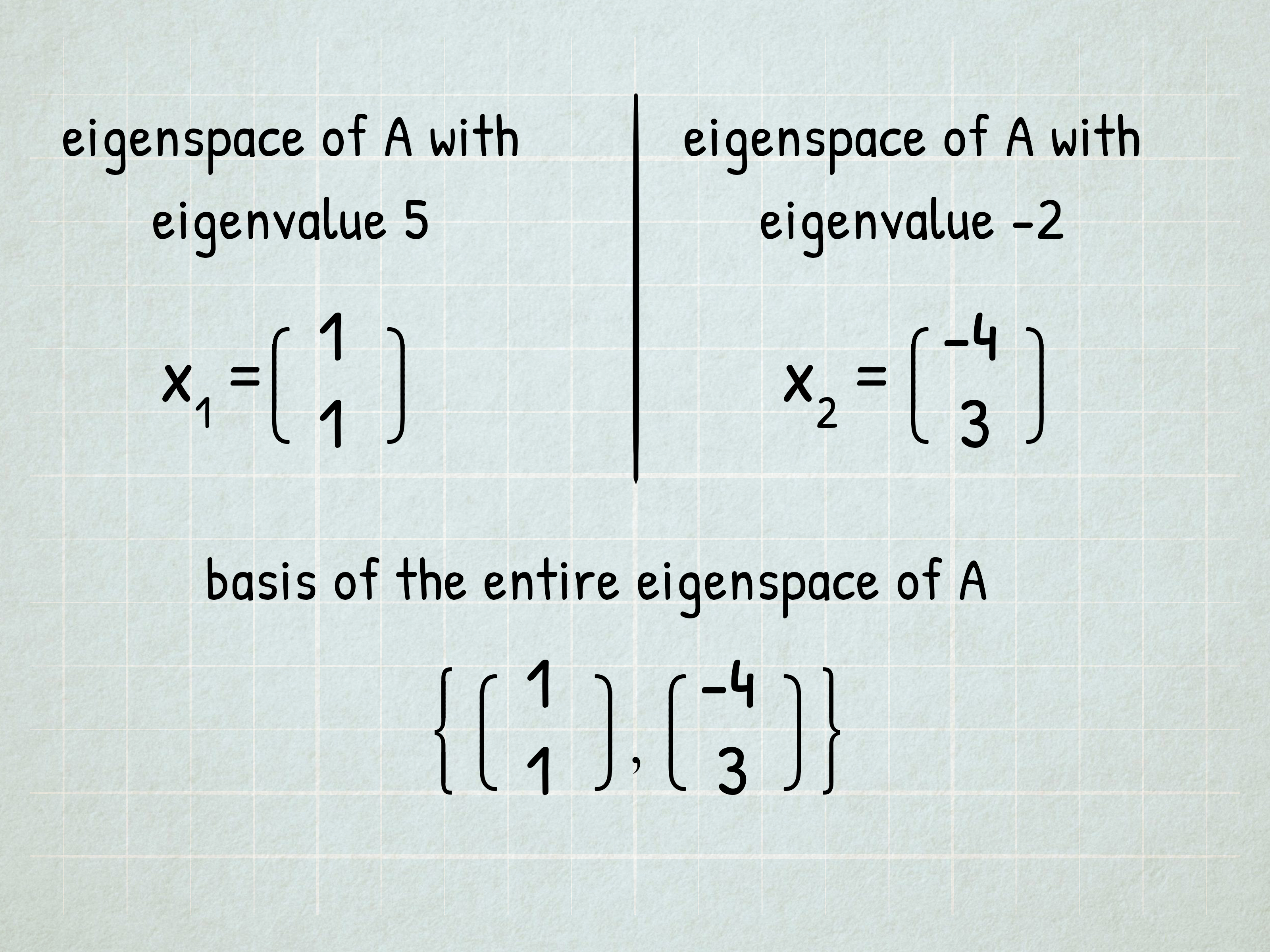
Repeated eigenvalues can be tricky. A repeated eigenvalue may or may not have enough independent eigenvectors to diagonalize the matrix. This is where eigenspaces and geometric multiplicity become important.
Eigenvalues, Eigenspaces, and Diagonalization
For each eigenvalue, the set of all corresponding eigenvectors, plus the zero vector, forms an eigenspace. You find this eigenspace by solving:
(A - λI)v = 0
If a matrix has enough linearly independent eigenvectors, it can often be diagonalized. Diagonalization rewrites a matrix in a simpler form, which makes repeated multiplication, solving systems, and analyzing transformations much easier.
This is one reason eigenvalues and eigenvectors are so powerful. They can turn a complicated matrix problem into a cleaner problem involving diagonal entries. In math terms, that is elegant. In student terms, that is fewer headaches.
Real-World Interpretation of Eigenvalues
Eigenvalues often describe rates, strengths, or magnitudes. In a vibration system, they may represent natural frequencies. In PCA, large eigenvalues indicate directions where data varies the most. In stability analysis, eigenvalues can show whether a system grows, decays, oscillates, or settles down.
That is why eigenvalues matter beyond pure math. They reveal behavior that may not be obvious just by staring at the entries of a matrix. A matrix can look ordinary, but its eigenvalues may tell a dramatic story.
Practical Experience: How to Get Better at Calculating Eigenvalues and Eigenvectors
From experience, the hardest part of learning how to calculate eigenvalues and eigenvectors in a matrix is not the definition. Most students can memorize Av = λv quickly. The real challenge is moving through the algebra without losing a sign, dropping a term, or suddenly wondering whether the Greek letter lambda has personally betrayed them.
The best way to improve is to start with small 2 × 2 matrices. They are large enough to show the full method but small enough that the determinant and factoring are manageable. Work through five or six examples by hand. Use matrices with clean integer answers first, such as symmetric matrices or triangular matrices. Triangular matrices are especially friendly because their eigenvalues are the diagonal entries.
One useful habit is to write every step clearly. Do not jump from A - λI directly to the final eigenvalues unless you are very comfortable. Write the determinant. Expand it. Simplify it. Factor it. Then solve it. This may feel slower at first, but it prevents mistakes and builds pattern recognition.
Another practical tip is to check every eigenvector. Many people stop after solving the nullspace, but checking with Av = λv catches errors immediately. If the left side and right side do not match, something went wrong. Maybe the eigenvalue was copied incorrectly. Maybe the row reduction had a sign error. Maybe the matrix saw you relax and chose violence.
It also helps to remember that eigenvectors can look different and still be correct. If your answer is [2, 1] and your textbook gives [4, 2], both are valid because they point in the same direction. If software gives decimals, it may have normalized the vector to length one. Do not panic. Compare direction, not just appearance.
For larger matrices, learn when to stop doing everything by hand. A 3 × 3 matrix can be a good exercise, but real applications often involve matrices with hundreds or thousands of rows and columns. In those cases, numerical tools are not cheating; they are the professional standard. The important skill is knowing what the software output means.
Finally, connect the calculation to geometry. When you find an eigenvector, picture it as a direction that survives the transformation. When you find an eigenvalue, picture it as the stretch factor along that direction. This mental image makes the topic feel less like symbol juggling and more like understanding how space moves.
Conclusion
Calculating eigenvalues and eigenvectors in a matrix follows a dependable process. Start with a square matrix, form A - λI, solve det(A - λI) = 0 for the eigenvalues, and then solve (A - λI)v = 0 for each eigenvector. The calculations can be detailed, but the idea is beautifully simple: eigenvectors keep their direction, and eigenvalues tell how much they scale.
Once you understand this process, matrices become easier to analyze. You can study transformations, solve systems, simplify repeated calculations, and understand important applications in data science, physics, engineering, and beyond. Eigenvalues and eigenvectors may look intimidating at first, but with practice, they become one of the most useful tools in linear algebra.